Matlab dispersion equations plot
Even when all the Maxwell equations are solved and clear results are obtained, it is useful to evaluate the plots of the functions. They can better show the behaviour and the features of the fields, and - above all - they are a main source for applications.
Plotting the dispersion equations
and finding a numerical value for their intersection is not a trivial task. Both Mathematica and Matlab are available for this kind of work. Here, Matlab (which is more suitable for designers) is used.
The original code has been published in this site. If it is offline, check out the local copies of the original files:
- original main script (local copy);
- original function for symmetrical modes (local copy);
- original function for asymmetrical modes (local copy).
These three files must be placed in the same directory, then the main script must be executed by Matlab (run by the GUI button or the F5 key).
However, several errors would arise in the case of a single intersection: the numerical values provided in the Matlab prompt do not correspond with the graphical values of the plots. The first are correct, while the plot is made in a wrong way: the $x$-axis and the $u \tan (u)$ curve are not properly scaled.
A modified version is here available for download:
- modified main script;
- modified function for symmetrical modes;
- modified function for asymmetrical modes.
The code is presented here:
%%%%%%%%%%%%%%%%%%%%%%%%%%%%%%%%%%%%%%%%%%%%%%%%%%%%%%%%%%%%%%%%%%%%%%%%%%%
% This code calculates the modes of a symmetric slab waveguide
%%%%%%%%%%%%%%%%%%%%%%%%%%%%%%%%%%%%%%%%%%%%%%%%%%%%%%%%%%%%%%%%%%%%%%%%%%%
%
% variables:
%   n1: cladding index
%   n2: core index
%   lr: wavlength (in vacuum, in micrometers)
%   d: vector with film thicknesses
%   pol: polarization state (1: TE, 2:TM)
%
% All length units are in micrometers (um),
% as well as wave vector units (1/um instead of 1/m
% for k0, kx, kz)
%%%%%%%%%%%%%%%%%%%%%%%%%%%%%%%%%%%%%%%%%%%%%%%%%%%%%%%%%%%%%%%%%%%%%%%%%%%
lr is the wavelength of the sinusoidal signal that should travel inside the waveguide, calculated in vacuum, as specified in the comments above. Please, note that:
-
all the quantities are in $\mu \mathrm{m}$. As a consequence of this, the output value of $k_z$ (whose standard unit of measurement is $1/\mathrm{m}$), will implicitly be expressed in $1 / (\mu \mathrm{m})$. This must be well considered, but it is not uncomfortable during computation, also when doing it by hand;
-
as in the original script, the cladding refractive index is
n1and the core refractive index isn2: this is the opposite convention with respect to the article notation.
global V

% waveguide parameters
% required parameters: n1, n2, a, lr
% be careful: n1 and n2 are swapped
n1=1.5;		% top region (the cover) refractive index
n2=1.6;		% core refractive index
a=3;		% half the waveguide core thickness, in um
lr=15;		% wavelength, in um
k0=2*pi/lr;
Specify here the numerical values that will be used during the whole execution. As pointed out in the article, only four parameters are necessary:
- the core half-thickness $a$;
- the vacuum wavelength of the signal $\lambda$;
- the refractive indexes of the two materials $n_1$ and $n_2$.
%%%%%%%%%%%%%%%%%%%%%%%%%%%%%%%%%%
%Equations:
%
%Dispersion equations
%   h=sqrt((n2*k0)^2-beta^2)
%   q=sqrt(beta^2-(n1*k0)^2)
%combine these 2 equations
%    h^2+q^2 = (n2^2-n1^2)*k0^2
%
%Mode equations
%   h*tan(h*a) = q (symmetric TE modes)
%   -h*cot(h*a)= q (antisymmetric TE modes)
%%%%%%%%%%%%%%%%%%%%%%%%%%%%%%%%%%%%%%%%%%%%%%
All the equations of the article are here recalled. The quantity beta is $k_z$.
% multiply both sides of the equations by a
% call x=ha, y=qa
%
% h*tan(h*d/2) = q  becomes x*tan(x)=y2
% (this y must be different than other ys, because each y
% represents a different curve and so a different function. This
% y is called y2)
% -h*cot(h*d/2) = q  becomes -x*cot(x)=y3
%
%   h^2+q^2 = (n2^2-n1^2)*k0^2 becomes x^2+y1^2 = a^2*k0^2*(n2^2-n1^2) = V
%

% normalized frequency
V=a*2*pi/lr*sqrt(n2^2-n1^2)
V is the variable representing the radius of the circumference $v$.
% break x up into 2 pi intervals
intervals=ceil(1.01*V)

%(1) plot the three equations
%   Dispersion equation
%   Symmetric modes
%   Antisymmetric modes
Here begins the first part of the script, when the plot only is performed. Even (symmetric) modes and odd (antisymmetric) modes are treated separetely.
figure('Name','Dispersion equations','pos',[350 25 750 750])
clf
hold 'on'
if intervals==1
    x=linspace(0, 1.5*V,1001);
All the elements needed for the plot must be built in a custom way, ad hoc to this specific problem. The distance between 0 and 1.5*V is split in 1001 parts (this will also be the $x$-axis resolution) and their positions are stored in the linear array x.
Like all the computational tools, Matlab represents numbers with a finite precision: its behaviour shows (in particular with such custom elements like the x array) all the consequences of this limited precision. This must always be taken into account, when performing the computations and when evaluating their results.
x=sort([x,V]);
The value of V is inserted between the elements of the previous linear array x, preserving the global order: in other words, this function sorts the concatenation of all the elements of x and V. This way, regardless of the above division of the $x$-axis in 1001 points, its array will always contain a value which is exactly the radius V.
I=find(x<=V);
% find the indexes of all the elements of x which are <= V
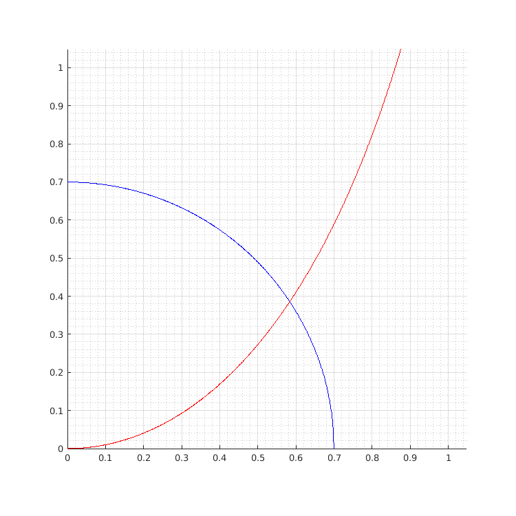
y1=sqrt(V^2-x.^2);
The quarter of circumference can be easily plotted if it is expressed as an ordinary function: the ordinate y1 must then be a function of the abscissa x.
    y2=x.*tan(x);     %symmetric
    y3=-x.*cot(x);    %antisymetric
    % argument of functions, variable in expressions
    % as well as plot() parameters must be considered
The characteristic equations $w = u \tan (u)$ and $w = -u \cot (u)$ are considered. In the script, the abscissa x represents $u$. $w$ is instead represented by two separate ordinate values y2 and y3 (this is necessary to generate two different plots).
    plot(x(I),y1(I),'b')
    plot(x,y2,'r')
    plot(x,y3,'g')
Note that the circumference, whose ordinate values are in the array y1, is plotted only for $x \leq v$ (x(I), y1(I)). The characteristic equations are instead plotted against the whole $x$-axis. b, r and g define the colors of the plots.
    grid
    axis image
    axis([0, max(x), 0, max(x)])
    grid minor
    hold 'off'

else

    for lp=1:intervals
        %only plot in pi/2 intervals to eliminate positive/negative changes
        x=linspace(pi/2*(lp-1),pi/2*lp,1001);
        x=x(2:end);
        I=find(x<V);
        y1=sqrt(V^2-x.^2);	%dispersion
        y2=x.*tan(x);		%symmetric
        y3=-x.*cot(x);		%antisymetric
        plot(x(I),y1(I),'b')
        plot(x,y2,'r')
        plot(x,y3,'g')
        % be careful to the default plot zoom: the function -x*cot(x) has
        % pi/2 = 1.57 as first root, but the x axis intersection may appear
        % slightly shifted. Zoom in for a better view.
    end
    grid
    axis image
    axis([0, pi/2*intervals, 0, pi/2*intervals])
    grid minor
    hold 'off'

end
The numerical results are obtained within the second part of the script, which begins in the subsequent line:
%(2) Calculate the symmetric modes
%number of symmetric modes
%tan(hd/2)=0
%   zero crossings every pi
%   hd every 2*pi up to V
n_sym= floor(V/(pi));
% number of available symmetric modes
x_sym=[];
for lp_sym=0:n_sym
    tmp=fminbnd('sym_modes_2',lp_sym*pi,lp_sym*pi+pi/2)
If the circle V intersects the tangent branch, it is between lp_sym*pi and lp_sim*pi+pi/2: not beyond, between lp_sim*pi+pi/2 and (lp_sym+1)*pi, because in this last range the tangent branch is below the $x$-axis.
The first separate file, sym_modes_2.m, is now recalled. It contains the definition of the function of the same name, sym_modes_2. This function is almost equal to err: it computes the difference between the tangent curve x*tan(x) and the circumference curve, sqrt(V^2 - x^2). When these curves coincide, that is when they intersect, a mode is found: so, a value of h and correspondingly a value of q and beta ($k_z$) can be obtained.
fminbnd finds the $x$-axis point, in the interval between lp_sym*pi and lp_sym*pi+pi/2, where the function sym_modes_2 is minimized, so where the intersection is obtained.
    x_sym=[x_sym,tmp]
    % concatenate tmp to the x_sym array
end
The third part deals with the odd modes with a similar procedure, but using the function asym_modes_2:
%(3) Calculate the anti-symmetric modes
%number of antisymmetric modes
%cot(hd/2)=0
%   zero crossings every pi/2
%   x every odd multiple of pi
n_asym= round(V/(pi));

x_asym=[];
if n_asym>0
    for lp_asym=1:n_asym
        tmp=fminbnd('asym_modes_2',pi/2+(lp_asym-1)*pi,pi+(lp_asym-1)*pi)
        x_asym=[x_asym,tmp]
    end
end

ha=sort([x_sym,x_asym]);
beta=sqrt((n2*k0)^2-(ha/a).^2)
neff=beta/k0
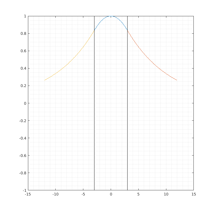
The field shape $e(x)$ is plotted as it appears in a $(x,y)$ section of the guide. After the beginning of the fourth part of the script, a new window is created and the abscissa range is divided into three regions, two belonging to the cover, one belonging to the core:
%(4) plot the mode fields
figure('Name','Mode fields','pos',[350 25 750 750])
x1=linspace(-a,a,101);
% core portion of x-axis
x2=linspace(a,4*a,101);
% cover portion of x-axis, right of core
x3=linspace(-4*a,-a,101);
% cover portion of x-axis, left of core

nn=0;

while nn<length(beta)
    nn=nn+1;
    subplot(length(beta),1,nn)

    if rem(nn,2)==0
    'odd'
Please, note that nn has already been increased before this check: it was initially 0 and now it is 1. This unit increment is systematic The first TE mode is always an even one, so in this script even modes will be related to odd values of nn and vice-versa.
        subplot(length(beta),1,nn)
        h=sqrt((n2*k0)^2-beta(nn).^2);
        q=sqrt(beta(nn).^2-(n1*k0)^2);
        % be careful: here, n1 is about the cover, n2 about the core
        C=sin(h*a)*exp(q*a);
        E1=sin(h*x1);
        % portion of plot inside the core
        E2=C*exp(-q*x2);
        % portion of plot right of the core. Note that the multiplication
        % of C and exp(-q*x2) gives the complete, correct expression:
        % sin(h*a)*exp(-q*(x2 - a))
        E3=-C*exp(q*x3);
        % portion of plot left of the core. x3 is already made up by
        % negative values of x
        plot(x1,E1)
        hold 'on'
        plot(x2,E2)
        plot(x3,E3)
        plot([-a -a], [-1 1],'k')
        plot([a a], [-1 1],'k')
        hold 'off'

    else    %even mode
        'even'
        h=sqrt((n2*k0)^2-beta(nn).^2);
        q=sqrt(beta(nn).^2-(n1*k0)^2);
        C=cos(h*a)*exp(q*a);
        E1=cos(h*x1);
        E2=C*exp(-q*x2);
        E3=C*exp(q*x3);
        plot(x1,E1)
        hold 'on'
        plot(x2,E2)
        plot(x3,E3)
        plot([-a -a], [-1 1],'k')
        plot([a a], [-1 1],'k')
        hold 'off'
    end
    grid minor
end

neff
This script produces the following output:
- the dispersion equations plot,
- the mode field distribution plot,
- the results in the Matlab prompt (run in version R2017a),
>> sym_waveguide_gh

V =

    0.6997


intervals =

     1


tmp =

    0.5838


x_sym =

    0.5838


beta =

    0.6413


neff =

    1.5311


ans =

    'even'


neff =

    1.5311
$ak_{x_1}$ is x_sym (and in this case, with only one interval between $0$ and $\pi / 2$, it coincides with tmp).
The same equations can be plotted with gnuplot with the following code:
set parametric
set trange [0:pi]
set yrange [0:2]
plot t, t*tan(t), t, sqrt(0.4896 - t**2)
The default viewer always shows the coordinates of the cursor, aiding in determining the position of the intersection. Through a graphic inspection of the output plot, a direct application of formulae and a calculator, the following results are obtained by hand:
- $v \simeq 0.6997$;
- $ak_{x_1} \simeq 0.5840$;
- $a | k_{x_2} | \simeq 0.3854$;
- $k_z \simeq 0.6413 \cdot 10^6 \ \displaystyle \frac{1}{\mathrm{m}}$;
- $n_{\mathrm{eff}} = \displaystyle \frac{k_z}{k_0} \simeq 1.5309$.
If the values from Matlab don’t perfectly match these ones in some cases, it is due to the different finite precision of the Matlab quantities and the hand calculator. Taking this into account, not only the Matlab script results are correct, but they are also coherent with the Matlab plots. To further verify this, and to better locate the position of the intersection in the Matlab plot, it can be downloaded in the svg format. The field plot is available in the same format, too:
-
dispersion equations (
svgfile); -
mode field distribution (
svgfile).
–

This work is licensed under a Creative Commons Attribution-ShareAlike 4.0 International License